05. June 2019
At some points, you have to dynamically generate mipmaps, i.e. downscale images. Either for textures, when they are not provided in the loaded image files or for render targets, e.g. to improve performance by running screen-space algorithms on downscaled render target versions or to find the average value of an image, e.g. like you have to for exposure eye-adaption based on the luminance of the rendered image.
In most cases (textures, rough approximations) you don’t care too much about correctness. Even when you need the average value of an image, the result often doesn’t have to be 100% accurate. Still, naive mipmapping will produce results that might be quite off, at least for non-power-of-two (NPOT) render targets. Think of a 1920x1080 window, where usually non-power-of-two framebuffer attachments are used. This is nothing new though, it’s one of the reasons textures traditionally always had a power-of-two size, but we will quickly look at the issue nonetheless.
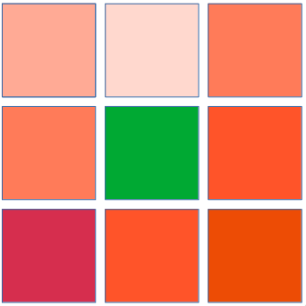
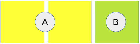
Let’s visualize it with a simple example: You have the image below, size 3x3.
You now generate the first mipmap level for that image. That mipmap level has size 1x1 (mipmap sizes are rounded down by convention in OpenGL and Vulkan). In vulkan generating the mipmap is usually done via a blit (notice how we are already using a linear filter here for best results):
vk::ImageBlit blit;
blit.srcSubresource.layerCount = 1;
blit.srcSubresource.mipLevel = 0;
blit.srcSubresource.aspectMask = vk::ImageAspectBits::color;
// srcOffset[1] is the size of the source
blit.srcOffsets[1].x = 3;
blit.srcOffsets[1].y = 3;
blit.srcOffsets[1].z = 1u;

blit.dstSubresource.layerCount = 1;
blit.dstSubresource.mipLevel = 1;
blit.dstSubresource.aspectMask = vk::ImageAspectBits::color;
// dstOffets[1] is the size of the destination
blit.dstOffsets[1].x = 1;
blit.dstOffsets[1].y = 1;
blit.dstOffsets[1].z = 1u;

vk::cmdBlitImage(commandBuffer,
    image, vk::ImageLayout::transferSrcOptimal, // mip 0: srcOptimal layout
    image, vk::ImageLayout::transferDstOptimal, // mip 1: dstOptimal layout
    {{blit}}, vk::Filter::linear);
But then you get this:

This is obviously not the mipmap we are looking for. The original image has quite some red pixels, why is the mipmap level only green? Well, the content for the pixel of the mipmap is determined via linearly filtering the source image. The destination pixel is perfectly in the center of the texture so to determine its contents, the center of the source image will be filtered. But since that is perfectly the center of the inner (center) pixel in the 3x3 image, no linear filtering will take place and the content of the mipmap is simply the center pixel of the original image. In other words: we discard 8/9 pixels and just copy one.
You may now think that the problem isn’t as bad when we start with a larger base image, but yes, it is. Because after some downsampling steps (in which we already discard quite some original pixels), we often enough end up with a 3x3 (or 2x3 or 3x2) mipmap which then, in turn, gets reduced to a 1x1 mipmap. So overall, a whole lot of pixels are discarded, even in the average case. So the value in the final 1x1 mipmap may be significantly different from the average value of the base image. It especially may only contain values from the center of the base image, discarding most of the rest.
Again, for conventional mipmaps (e.g. an albedo texture) this shouldn’t really be a huge problem since a rough approximation is usually enough, the mipmap levels don’t really have to contain the average. We can even improve it a bit by always using an even source size when blitting (i.e. intentionally discarding the last row for uneven sizes). In the example above, we would blit the 2x2 first pixels of the source image (discarding the last row/column) to the 1x1 mipmap, linear filtering works in that case and we only end up with 5/9 discarded pixels.
But what if we do this whole mip-mapping only to get the average of an image on the GPU? This is the case for simulated eye-adaption were we compute the average luminance (or, more correctly: average of log(luminance), i.e. we want the geometric mean) of the rendered image to adjust the exposure of our HDR tone mapping. When you use the naive mipmap approximation it’s quite easy to notice that the adaption only takes a fraction of the screen into account. Additionally, the error will be highly dependent on the image size. That means when resizing the render target (i.e. the window), in one frame you might have an average luminance of 0.05 and in the next frame one of 0.2, although only one row of pixels was added/removed, i.e. the real geometric luminance mean has only changed insignificantly. Those properties are usually not acceptable.
So let’s do something fun: implement a compute shader that does what we want even faster than generating a mipmap. We aren’t after all interested in the mipmaps, this is more of a hack, to begin with. We just want the average value of a (possibly non-power-of-two) texture. How hard can it be…?
Since the images will usually be too large to compute the average in a single pass and since we want to make good use of the parallel hardware we get on a GPU, we will use something that resembles mip-mapping except that we use a larger downscale factor (e.g. reducing the size by factor 8, 16 or 32 instead of just 2 in every pass). We will additionally downscale correctly, i.e. are not discarding any pixels.
Requiring that the workgroup size is the same in x- and y-direction (i.e. blocks and workgroups are quadratic) simplifies the implementation a lot and there shouldn’t be a reason to choose something else. For the sake of simplicity and visualization, let’s fix the work group size (in each dimension) to s = 4 for the rest of the article. For a real implementation 8 or 16 tended to be a bit faster on my hardware. The border conditions are where this gets somewhat ugly. My first idea was to weigh the border pixels, i.e. always remember how much the last row/column is worth average-wise:
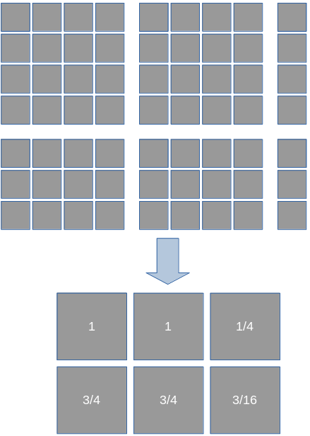
After this iteration, we would store (\frac{1}{4}, \frac{3}{4}) as the weight of the last pixel row/column. In the next iteration that weight would be applied to the values read from the last row/column. It would additionally used when diving by the number of pixels sampled, e.g. the last row/column wouldn’t be counted as one but as their weight. That algorithm worked, but in a second code iteration I went with a way that is somewhat easier to implement: for the sake of average calculation we just virtually pretend that the original image’s size is a power of our per-dimension work group size s and we, therefore, have only full blocks in all reduction steps.
When calculating the average, sum up all pixels in the block and then always divide by the s * s (i.e. the number of sampled pixels in a full block), even if block contained fewer pixels. You can imagine this as “summing up 0” for the pixels outside of the input image size. And then - at the end, when the average of the whole image was calculated like that - we will account for the 0-pixels in that average with a correction-factor that is simply calculated like \frac{npo(width, s) * npo(height, s)}{width * height} where npo(x, b) is the smallest power of b greater or equal to x: npo(x, b) = b^{\left\lceil\log_b x\right\rceil} So the correction factor is the virtual number of pixels we sum up (including the zeroes) divided by the real number of pixels.
Although not exactly a formal proof (have yet to see one in a graphics post), you can see that this is correct like this: Take an average of a series of n values v_i \frac{1}{n}\sum_{i=1}^{n}v_i and now add k zeroes to the series and again calculate the average: \frac{1}{n + k}\sum_{i=1}^{n}v_i (obviously the zeroes have no effect on the sum). If you now want the average without the artificial zeroes, you just have to multiply that with \frac{n + k}{n}, which is exactly our correction factor above.
With border conditions out of the way, the next question is which mip targets do we store to/read from? When s = 4 we reduce the image dimensions by factor 4 in each step so we could theoretically only use every other mip level. Except that mip level sizes are rounded down and we need rounding up (see the reduction sketch again, we also store not-full blocks). So in some cases, when the mip level size is too small, we have to use the previous mip level. In practice, this will probably only happen once since after that we got plenty of room in our mipmaps. Pseudo-codish it looks like this:
s = 4; // our group size per dimension
shift = log2(s); // mipmap jumping count
src = 0; // current source mip level
dst = shift; // current destination mip level
srcWidth = image.width;
srcHeight = image.height;
while(iwidth > 1 || iheight > 1) {
    // compute mip level size of level dst
    mipWidth = std::max(image.width >> dst, 1u);
    mipHeight = std::max(image.height >> dst, 1u);

    // compute the needed size (rounding up!)
    dstWidth = (srcWidth + s - 1) / s;
    dstcHeight = (srcHeight + s - 1) / s;

    // check if we have to back one level
    if(iwidth > mipWidth || iheight > mipHeight) {
        --dst;
    }

    // run compute shader here
    // it reads from mip level src
    // writes to mip level dst
    // (dstWidth, dstHeight, 1) invocations are needed
    // we have to pass (srcWidth, srcHeight) to the shader

    src = dst;
    srcWidth = dstWidth;
    srcHeight = dstHeight;
}
With all that ugly groundwork out of the way, let’s get to the beautiful part: the parallel reduction shader. It needs the following inputs:
srctextureSize doesn’t work here since the real size of that mip level may be larger than the sub-image we have written to. We pass that as push constant (uniform buffer objects work too but that requires us to keep a separate ubo for every pass and since this value only changes every time the original image size changes - in which case we have to re-record command buffers anyways - a push constant is the best solution here). In the code above this is simply (srcWidth, srcHeight).And it writes to the dst mipmap level Every workgroup will reduce one s x s block to size 1 - computing its average - and write that value to the dst mipmap level, the output pixel is the workgroup ID (gl_WorkGroupID). Let’s look at the shader. This is already the optimized version, with various ideas from nvidia’s presentation on optimizing parallel reduction as well as own ideas we will discuss shortly already applied. There are probably still some optimization opportunities left though.
#version 450
// we assume that x and y wor group sizes are the same.
// There is no reason why we should choose something else and it
// simplifies the computation here tremendously
layout(local_size_x_id = 0, local_size_y_id = 0) in;
// The source mipmap level with a linear sampler
layout(set = 0, binding = 0) uniform sampler2D inLum;
// The destination mipmap level
layout(set = 0, binding = 1, r16f) uniform writeonly image2D outLum;
layout(push_constant) uniform PCR {
uvec2 inSize; // size of valid pixels in the source level
} pcr;
// constant for all invocations
const uint size = gl_WorkGroupSize.x; // == gl_WorkGroupSize.y
vec2 pixelSize = 1.f / textureSize(inLum, 0);
// contains the current summed-up luminance
shared float lum[2 * size][2 * size];
// Loads the from the given pixel but makes sure to never sample
// out-of-bounds.
float load(vec2 pixel) {
// return 0 when outside of image.
// don't make a multiplication or something else out of this
// since we might sample values like inf or nan from the texture
// outside of inSize
if(any(greaterThan(pixel, vec2(pcr.inSize)))) {
return 0.f;
}
// on the image edge we might have to sample two (or even just
// one in case of corner) instead of the normal 4 pixels.
// Weigh them accordingly and make
// sure we never sample outside of the valid region of
// input mip level (gvien via pcr.inSize)
float fac = 1.f;
if(pixel.x > pcr.inSize.x - 0.5) {
fac *= 0.5f;
pixel.x = pcr.inSize.x - 0.5;
}
if(pixel.y > pcr.inSize.y - 0.5) {
fac *= 0.5f;
pixel.y = pcr.inSize.y - 0.5;
}
return fac * texture(inLum, pixel * pixelSize).r;
}
void main() {
// 1: compute base of pixels this invocation is responsible for
uvec2 l = gl_LocalInvocationID.xy;
vec2 pixel = 4 * gl_GlobalInvocationID.xy; // top-left of sampled pixels
pixel += 1;
// 2: load responsible pixels
lum[2 * l.x + 0][2 * l.y + 0] = load(pixel + vec2(0, 0)); // A
lum[2 * l.x + 1][2 * l.y + 0] = load(pixel + vec2(2, 0)); // B
lum[2 * l.x + 0][2 * l.y + 1] = load(pixel + vec2(0, 2)); // C
lum[2 * l.x + 1][2 * l.y + 1] = load(pixel + vec2(2, 2)); // D
// 3: reduction loop
for(uint isize = size; isize > 0; isize /= 2) {
barrier();
// sum up in tiles
if(l.x < isize && l.y < isize) {
lum[l.x][l.y] += lum[isize + l.x][l.y]; // a, b, c, d
lum[l.x][l.y] += lum[l.x][isize + l.y]; // e, f, g, h
lum[l.x][l.y] += lum[isize + l.x][isize + l.y]; // i, j, k, l
}
}
// 4: first invocation in group writes average back
if(l.x == 0 && l.y == 0) {
// divide by the pixel count of the full block
float avg = lum[0][0] / (4 * size * size);
imageStore(outLum, ivec2(gl_WorkGroupID.xy), vec4(avg));
}
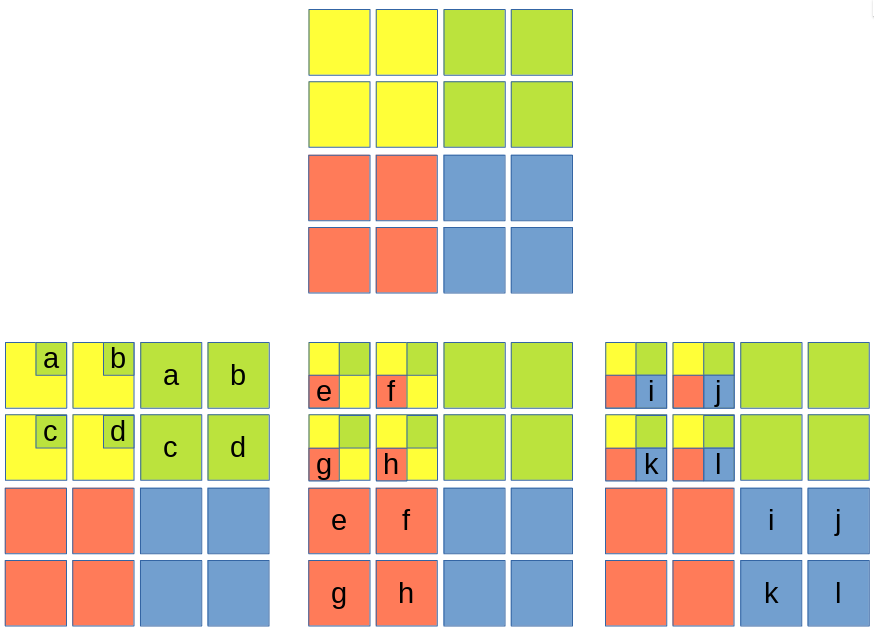
}The basic structure is already documented in the code, just follow the numbered comments. The reduction loop always sums up 3 tiles onto the base tile. In the sketch below, multiple colors in one field mean that they have been summed up (the sketch is ignoring the optimizations discussed below regarding group size, it displays the first reduction iteration for a block of size 4 per dimension):
Before each reduction iteration, a barrier is needed. With Vulkan semantics for glsl, no memoryBarrierShared is needed here since barrier automatically performs that. See the GL_KHR_vulkan_glsl and the spirv specifications for more details. For OpenGL it might be needed, see https://stackoverflow.com/questions/39393560. Also note that there cannot be any early returns, since then barriers become undefined behavior.
Let’s start with the two most important optimizations that make this implementation a bit different from the more theoretical, simplistic above:
lum is twice the size in every dimension (four times the size in total) and every invocation fills in 4 of those values.sampler2D must also have a linear sampler for that to work. So In total, every invocation (not at the border) will read (2 * 2) * (2 * 2) = 16 values from the texture instead of just 1. This helps keeping the number of invocations down that would just sit idly during most of the reduction loop. During the first reduction iteration, all invocations will be active (that’s what optimization 1 is for, why our shared buffer has twice the size in every dimension). For non-border invocations the sampling works like this (load is basically just one texture access at the given coordinates):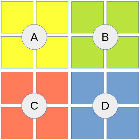
For invocations that have to sample pixels beyond the input image size, load will return 0, as described in the theory. For border samples, it might move the sampled position by 0.5 in each dimension to make sure the last row/column pixels are sampled but nothing beyond it. It then applies a factor that makes the function overall behave as if it just normally sampled the given position but everything beyond the input texture size is 0. E.g. for the bottom right corner of the input mip level, with width \% 4 = 3 and height \% 4 = 1 it might look like this (load for C, D will return 0):
Note that we could alternatively achieve this with clearing the used mip levels to black once and bind a sampler with clampToBorder addressing mode and a black border. This would simplify the shader a bit, we basically move the responsibility for clamping into the sampler, i.e. onto the GPU. The clear might hurt performance a bit but shouldn’t have a big impact so this is a viable alternative.
The load function is only that explicit for understanding and documentation reasons. With some glsl foo we can reduce it to this:
float load(vec2 pixel) {
    vec2 dist = clamp(pcr.inSize - (pixel - 0.5), 0, 1);
    float fac = dist.x * dist.y;
    vec2 uv = min(pixel, pcr.inSize - 0.5) * pixelSize;
    return fac * texture(inLum, uv).r;
}
Note how we still never sample from a location outside of pcr.inSize (not even via linear sampling) since that might introduce nan to the system - in which case the whole average computation would get nan’ed.
But now that every invocation reads from 16 pixels we have to adapt our algorithm for selecting matching mip levels accordingly. This is rather trivial though, instead of using s as block width and height, we simply use 4 * s. That has an effect of shift in the pseudo code above as well as the previously discussed correction factor (we now need the next power of the block size, i.e. 4 * s).
The result looks like this (starting with full HD, s = 8):
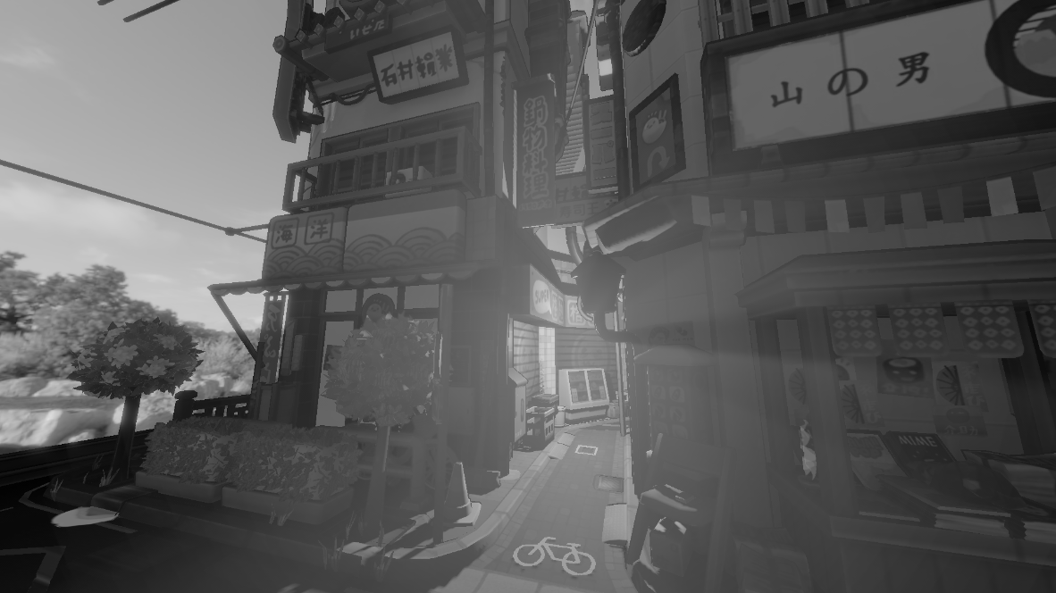


In each level, we reduced the mipmap size by 4 * s = 32 in each dimension, but in comparison to standard mipmap sizes we round up (i.e. 60 / 32 \to 2). You may notice that e.g. the bottom pixels of the 2x2 level or the pixel of the final level aren’t really the average when compared to the corresponding blocks in the previous level. But this is due to our “sample 0 beyond the input image” approach. The border pixels may have values that are nearer 0 due to that (the black pixels here are negative, remember that we are dealing with log(luminance), so the pixels nearer 0 are brighter in this case). But this is fixed with the correction factor at the end! In this case, it’s
\frac{npo(1920, 32) * npo(1080, 32)}{1920 * 1080} \approx 517
The value of the final mip level is \approx -0.01 so we get \approx -5.17 as average log(luminance) value, i.e. 0.02 as geometric mean of the luminance, which is correct (as this value is in linear space, i.e. not yet gamma corrected and the original image was indeed quite gloomy). You can see here already that forgetting to apply the correction factor will result in completely wrong results.
Also note that the unused regions of the mip levels can be left uninitialized, as we never access them. In this case, it’s pure coincidence that the GPU memory seems to contain a uniform value, I’ve also seen (and debugged…) cases where the memory contained values that equaled float NaN’s or infinities that completely messed up the calculation. The current code is careful to never sample them in any way.
Most of those ideas should be properly benchmarked, most will probably only result in an insignificant change or even in a worse result.
loadFor Vulkan, don’t forget to insert image memory barriers between the passes, you probably also want to transition the old destination (new source) mip level from general to shaderReadOnlyOptimal layout there. After all passes were executed and the last one wrote the final average to the last mipmap level, it can be copied from that to a buffer (or otherwise processed). But don’t forget the correction factor!
We could also just use a power-of-two render target (just round up the window size to the next power-of-two) and then use the old mipmapping algorithm. But rendering that in its full size might not always be possible or require additional workarounds (e.g. in Vulkan all framebuffer attachments must have the same size). Additionally, when simply rendering a fraction of it, adaptions like the correction factor above are needed as well after mipmapping. You furthermore need a clear to black at the beginning which might not have been needed otherwise (depending on when you generate the luminance rendertarget). So, given that the compute shader alternative should be faster in pretty much all cases, uses less memory and doesn’t require any hacks, it should probably be preferred. The only reason I could think of not using compute shaders here is if your luminance format isn’t supported for storage images (but e.g. the r16f format is guaranteed to be supported by Vulkan).